LandOffer
Data & Decisions
Estimate an Experiment's Duration Before You Commit a Release Date
A synthetic fixed-horizon binary-outcome plan uses a 10% baseline, a 2-percentage-point difference, two-sided 5% alpha, and 80% power to estimate 3,841 users per group. Executed normal-approximation and calendar checks translate 250 versus 125 users per group daily into 21-day versus 35-day proposals, plus 24-hour outcomes and two analysis days; checkpoints do not promise effects or approval.
Estimate an experiment’s duration from its metric, baseline, meaningful effect size, statistical method, and eligible new participants before promising a release date. Translate the required sample per group into traffic at the actual allocation, then add the observation window, calendar coverage, and analysis work. Treat the calculated date as a conditional analysis checkpoint; it does not promise an effect, significance, or release approval.
This LandOffer.ai guide supplies a complete synthetic planning case and a revised plan when traffic halves. Deterministic Python calculations verify the sample approximation and calendar arithmetic. No experiment was launched, no analytics account was accessed, and no calculator interface was tested. The figures illustrate planning assumptions rather than a forecast for an existing product.
Define the question and experimental unit first
The fictional LabelNest product lets a person create a reusable label template. Product owner Mei wants to test a simplified editor. The primary metric is whether an eligible user completes a first template within 24 hours of the first experiment exposure. Each user contributes one binary outcome, success or failure, and remains assigned to the same variant.
The planning population is newly eligible users, not page views or every visit. Returning to the editor five times does not create five independent participants. Repeated measurements, account-level assignment, interactions between users, or a different outcome type would require a design that accounts for those features rather than recycling this calculation.
Mei proposes November 20, 2026, as a release target. Analyst Arun records it as a requested date and checks feasibility before exposure begins. No actual team has accepted the fictional schedule. Staffing, holidays, platform capacity, and release approval remain outside the calendar arithmetic below.
The first completed planning asset starts with the following fixed assumptions:
| Input | Explicit synthetic assumption |
|---|---|
| Primary outcome | First template completed within 24 hours; one outcome per user |
| Baseline completion rate | 10% in the intended eligible population |
| Minimum detectable difference for planning | 10% to 12%: 2 percentage points, or 20% relative lift |
| Groups | Two independently randomized groups, equal allocation |
| Significance level | Two-sided 5%, one primary comparison |
| Target power | 80% at the specified 2-point difference under the planning model |
| Eligible new users | Forecast 1,000 per calendar day before experiment allocation |
| Traffic assigned to experiment | 50% of eligible users; split equally between control and treatment |
| Timing convention | UTC calendar days; exposure begins November 3 at 00:00 |
The baseline needs to match the metric’s denominator and observation window. A rate calculated from all visits or incomplete 24-hour outcomes would be a poor input for this user-level design. In a real plan, retain the baseline extraction period, exclusions, and uncertainty instead of treating a rounded dashboard percentage as a timeless constant.
Calculate sample per group without promising detection
Evan Miller’s sample-size tool labels sample size per variation and distinguishes absolute from relative effect size. Those details matter when moving an estimate into a schedule. A 2-percentage-point increase from 10% is a 20% relative increase; a 2% relative increase would instead mean 10% to 10.2%, a much smaller difference.
For this example, the local script evaluates the two-sided normal-approximation power equation documented in Minitab’s two-proportions methods. It searches for the smallest integer sample per group reaching the target. The documented two-sided power-formula image was inspected and evaluated locally; Minitab software was not run.
The result is 3,841 users per group, or 7,682 total. At that integer, the evaluated approximate power is about 80.002%; at one fewer per group it falls below 80%. A separately evaluated common closed-form normal approximation rounds up to the same sample size. The two calculations agree on the rounded planning sample; neither establishes that a real experiment satisfies the model’s assumptions.
This calculation assumes independent binary outcomes and uses no continuity correction. A platform’s implementation, a sequential design, an exact method, unequal allocation, multiple comparisons, clustered assignment, or a different metric can require a different plan. Match the calculator and stopping method to the analysis you intend to perform.
Power is conditional on a specified true effect and model. It does not mean the feature has an 80% probability of working, or that a significant result will appear by the scheduled day. A real effect smaller than the planning difference can remain hard to distinguish from noise. An experiment can also yield evidence of harm or an inconclusive result.
As a sensitivity check, changing the assumed comparison from 12% to 11% raises the same method’s requirement to 14,751 per group. That is not a reason to choose a larger effect merely to make a deadline fit. The detectable effect should reflect a meaningful decision and a feasible design, with the compromise made explicit.
Convert eligible traffic into a calendar plan
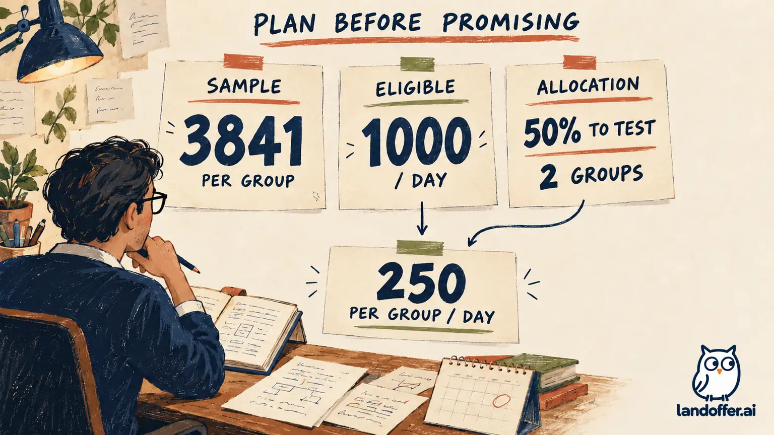
Apply the allocation before dividing sample by traffic. From 1,000 newly eligible users per day, 50% enter the experiment: 500 total. Splitting those equally gives 250 users per group per day. Dividing 3,841 by 250 gives just over 15 days, rounded up to 16 whole days of forecast sample accumulation.
The 16-day sample forecast leaves the calendar and outcome windows unresolved. The fictional team chooses a preplanned 21-calendar-day exposure period to include three complete weekly cycles. This is a case-specific choice, not a universal rule that every experiment needs three weeks. Microsoft’s PlayFab experimentation guidance calls attention to comparable periods, seasonality, sufficient duration, and the population allocated to an experiment.
| Base-plan stage | Calculation or assumption | Conditional checkpoint |
|---|---|---|
| Required sample | 3,841 users per group | A minimum planning requirement, not a guaranteed outcome |
| Forecast accumulation | 250 per group daily; 16 whole days to reach the requirement | Does not yet cover the chosen full-week period |
| Chosen exposure period | 21 calendar days beginning November 3 at 00:00 UTC | Exposure stops November 24 at 00:00 UTC, exclusive |
| Expected sample at that rate | 21 × 250 = 5,250 per group | Forecast only; validate actual eligible enrollment |
| Outcome maturation | Allow the final exposed users their full 24-hour outcome window | Complete by November 25 at 00:00 under the timing assumptions |
| Analysis allowance | Two calendar days after outcomes mature | Earliest arithmetic checkpoint: November 27 at 00:00 UTC |
The November 20 release request is earlier than this checkpoint. Even a favorable-looking early result would not make the uncompleted exposure and outcome windows disappear. Arun’s response is to revise the plan before launch, not to promise that the test will deliver a winner sooner.
The stopping plan must state how the chosen duration and minimum valid sample interact. Here, the proposal is the 21-day period with at least the planned sample in each group and complete outcomes before analysis. If actual enrollment is insufficient, the preplanned protocol needs a defensible next step; silently extending a conventional fixed-horizon test after inspecting its effect is not the same design.
Audit the traffic forecast against the entry rule before turning it into daily sample. Exclude already assigned participants from new enrollment, account for rollout ramps, and inspect day-of-week variation. If an audience filter is applied after assignment in a way affected by treatment, its apparent volume can also conceal a biased comparison. The simple constant-rate calculation here assumes those issues have been resolved; it does not verify them.
Calendar arithmetic also does not reserve people. The two analysis days include every calendar day in this simplified model. They are not verified business days or staffed review appointments. Data-ingestion delays beyond the stated outcome window, instrumentation problems, and approval lead time could move the actual decision later.
Revise the plan when the traffic forecast halves
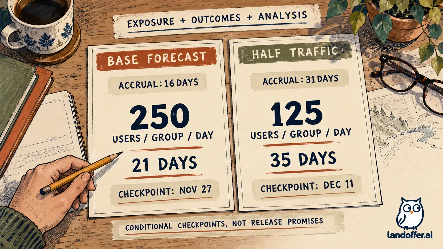
Before exposure begins, the fictional team learns that only 500 newly eligible users per day are expected. The experiment still receives 50%, and the two groups still split that traffic equally. Each group now receives 125 users per day. The sample requirement stays 3,841 because the metric, effect size, and statistical assumptions have not changed.
This is the second completed planning asset: a revised forecast and decision record, not an observed slowdown from a real experiment.
| Planning element | Original forecast | Half-traffic forecast |
|---|---|---|
| Eligible new users daily | 1,000 | 500 |
| Total experiment users daily | 500 | 250 |
| Users per group daily | 250 | 125 |
| Whole days to accumulate 3,841 per group | 16 | 31 |
| Chosen full-week exposure period | 21 days | 35 days |
| Forecast sample per group at chosen stop | 5,250 | 4,375 |
| Exposure stop, exclusive | November 24 at 00:00 UTC | December 8 at 00:00 UTC |
| Outcomes mature under 24-hour rule | November 25 at 00:00 UTC | December 9 at 00:00 UTC |
| Earliest checkpoint after two analysis days | November 27 at 00:00 UTC | December 11 at 00:00 UTC |
Mei’s fictional planning response records: “Do not commit November 20 as an evidence-based release date. Keep the stated outcome and 2-point planning difference. If we run the equal-allocation design with the lower forecast, use the 35-day proposal and December 11 arithmetic checkpoint, subject to valid data, staffing, and approval. Decide before launch whether that timeline is worth the opportunity cost.”
Other options deserve explicit evaluation: changing the audience, allocating more eligible traffic, narrowing the question, or choosing another research method. Each can alter risk or what the result generalizes to. This example does not assume more traffic is available, lower the power target to hide the delay, or convert the requested deadline into permission to stop early.
Preserve the assumptions through the release discussion
Twenty-two executed Python checks retain the sample search, power boundary, independent rounded approximation, allocation arithmetic, date additions, and smaller-effect sensitivity. These deterministic checks establish the stated calculations, not experiment outcomes, platform results, or future enrollment.
Before launch, assign owners for the eligibility query, assignment and exposure logging, outcome completion, and analysis method. Verify that people are counted once, treatment persists as intended, and instrumentation does not exclude one variant unevenly. A large sample cannot compensate for a broken comparison or a metric that measures a different action from the one specified.
Keep guardrails and their decision rules visible too. A primary binary completion calculation does not automatically power every safety, latency, revenue, or subgroup measure. If additional comparisons are decision-critical, have the analysis owner account for their method and multiplicity rather than treating this one sample size as blanket statistical coverage.
Agree on the possible analysis outcomes before the exposure period starts. A favorable estimate with wide uncertainty may not justify a release, and a non-significant result does not establish that the variants are identical. The final decision should consider the effect estimate, uncertainty, guardrails, and practical costs under the chosen method, not merely whether the calendar reached a promised date.
Separate operational monitoring from a claim of statistical success. Teams may need to stop for serious technical harm under predeclared rules. That is different from repeatedly looking for a favorable p-value and declaring the planned effect detected as soon as one appears. Sequential monitoring requires a method designed for it, not just a new label on repeated fixed-horizon checks.
For your next experiment proposal, show sample per group, eligible allocated users per day, exposure period, outcome maturity, and analysis allowance in one table. Put the assumptions beside the requested release date and state what could move the checkpoint. More practical data guides are available from LandOffer.ai.